Are line lengths in R more lognormal than in python?
Jake van der Plas recently analyzed the distribution of line lengths in the source code of Python packages (I highly recommend reading this post!). In particular, he investigated the influence of th 79-character limit which is imposed by the PEP8 style guide on programming habits and style conventions. He found out that this strict recommendation causes a bump in the distribution at or near the 79-character limit. He also found differences in this distribution between packages and concluded that some packages follow the style guide stricter than others.
This observation inspired me to perform a similar analysis of the source code of R packages. I regularly use Python as a general purpose programming language, for purposes like image analysis, sorting of files and other tasks. In R, on the other hand, I am much more a user than a programmer, with a focus on data analysis, modeling and visualization. Jake vdPs analysis inspired me to reproduce this work in R, with the purpose to analyze line lengths in R code. From this task, I hope:
To become more familiar with R as a programming language
To observe how the lack of a strict style guide in the R world affects the distribution of line lengths.
To observe whether there are style differences w.r.t to line length between packages (and developers)
Counting lines in the dplyr package
Unlike in Python, the source code of installed R packages is not directly available (if it is, I haven’t found it). For this analysis, I have therefore downloaded package sources from cran manually.
First, we need a function that reports lines and their lengths in an arbitrary R package. In python, this would be straigthforward (for me), in R, I lack foundations. Since I work within the tidyverse, this function should return a dataframe with the columns Package, Line and Length. After some base R exercises, I produced the following function:
library(tidyverse)
file_to_df <- function(filename){
  # read a file line-by-line into a dataframe
  df <- as_data_frame(readr::read_lines(filename))
  df
}

line_lengths <- function(package){
  # this function reads lines and counts their length in all R scripts in a given directory
  # For now, the source code of the package needs to be downloaded manually

  # list all R files in path
  pkg.path = file.path("../../src",package)
  filelist = list.files(path = pkg.path,
                       pattern = '.*\\.R$', # all files that end with .R
                        full.names = T, # for convenience: full path
                        recursive = T)

  # for each R file: read lines and count length
  # for loops are evil, we use purrr::map
  dfs <- purrr::map(filelist, file_to_df)

  df = bind_rows(dfs) %>% ## merge dataframes
    mutate(Package = package) %>% # insert the package name, for convenience
    mutate(line_length = nchar(value)) # determine line length
  return(df)
}
With the function line_lengths, we can now proceed with the fun part and investigate the line lengths in dplyr:
dplyr.lines <- line_lengths("dplyr")

dplyr.lines %>%
  ggplot(aes(x=line_length)) +
  geom_histogram(binwidth = 1, color = "dark gray", fill="light gray")
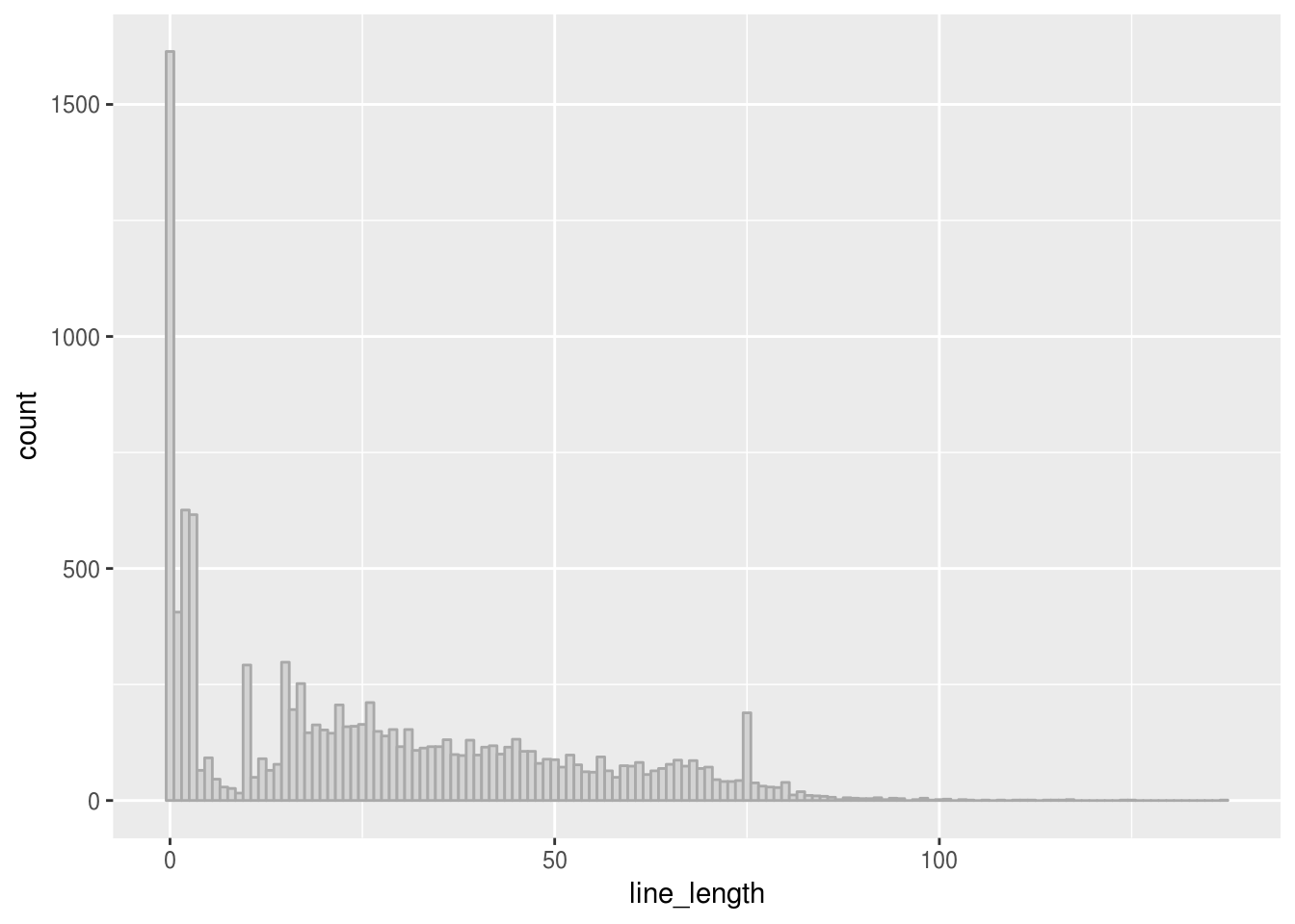
We observe two distinct peakes in the histogram, one for empty lines and one for lines with a length of 75. We investigate the latter:
dplyr.lines %>%
  filter(line_length==75) %>% select(value)
## # A tibble: 189 x 1
## value
## <chr>
## 1 ## ----setup, include = FALSE----------------------------------------------
## 2 "## ---- results = \"hide\"------------------------------------------------
## 3 ## ---- eval = FALSE-------------------------------------------------------
## 4 ## ------------------------------------------------------------------------
## 5 ## ---- eval = FALSE-------------------------------------------------------
## 6 ## ---- eval = FALSE-------------------------------------------------------
## 7 "## ---- results = \"hide\"------------------------------------------------
## 8 ## ------------------------------------------------------------------------
## 9 ## ------------------------------------------------------------------------
## 10 ## ------------------------------------------------------------------------
## # ... with 179 more rowsApparently, comment lines are often dash-filled to a line length of 75.
What is it with those lines of length 2?
dplyr.lines %>%
  filter(line_length==2) %>%
  count(value)
## # A tibble: 7 x 2
## value n
## <chr> <int>
## 1 2
## 2 )) 1
## 3 }) 370
## 4 #' 249
## 5 ## 2
## 6 x1 1
## 7 x2 1Many of these lines are closing parentheses - this is something which is rarely observed in the python world.
Following Jvdp, we focus further analysis on unique lines only, in order to remove boring boiler plate code:
dplyr.lines %>%
  distinct() %>%
  ggplot(aes(x=line_length)) +
  geom_histogram(binwidth = 1, color = "dark gray", fill="light gray")
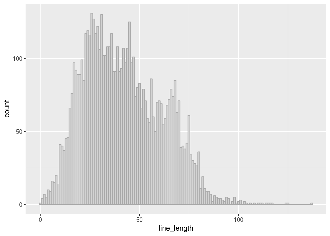
This looks much more like the kind of distribution which we expect after having read Jake vdP’s article. There appears to be a bump in line lengths around 65-70 characters, which may well result form personal preferences and editor window widths. Otherwise, the distribution looks fairly smooth and approximately lognormal.
More packages
We extend the analysis to the popular ggplot2 library:
ggplot.lines <- line_lengths("ggplot2")

ggplot.lines %>%
  distinct() %>%
  ggplot(aes(x=line_length)) +
geom_histogram(binwidth = 1, color = "dark gray", fill="light gray") 
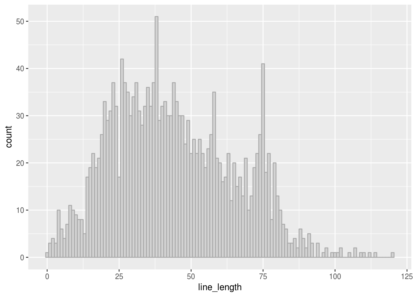
The distribution of line lengths in ggplot2 has a roughly similar shape to dplyr. This comes as no surprise, since both packages share the same developer. However, we observe a peak at line length 75, maybe enforced by an editor limit on line length, and a curious peak at length 38.
ggplot.lines %>%
  distinct() %>%
  filter(line_length==38)
## # A tibble: 51 x 3
## value Package line_length
## <chr> <chr> <int>
## 1 rng <- range(data$x, na.rm = TRUE) ggplot2 38
## 2 ...) { ggplot2 38
## 3 stat_density_common(bandwidth = 0.5) ggplot2 38
## 4 data.frame(x = d$x, density = d$y) ggplot2 38
## 5 ggplot(mpg, aes(displ, fill = drv)) + ggplot2 38
## 6 # Place panels according to settings ggplot2 38
## 7 panels <- matrix(panels, ncol = 2) ggplot2 38
## 8 panels <- matrix(panels, ncol = 1) ggplot2 38
## 9 ## Recalculate as gtable has changed ggplot2 38
## 10 trans = scales::as.trans(trans), ggplot2 38
## # ... with 41 more rowsI don’t have a proper explanation for this peak - this may well be a random finding and have no reason at all.
More developers
R has no general style guide. It is therefore quite likely that developers rely on personal preferences, e.g. for line length. We extend our analysis to two machine learning packages, caret and [mlr](https://mlr-org.github.io/.
Also, we modify the visualization by using a facet plot.
mlr.lines <- line_lengths("mlr")
caret.lines <- line_lengths("caret")
df.all <- bind_rows(ggplot.lines, dplyr.lines,
                    caret.lines,mlr.lines)

df.all %>%
  distinct() %>%
  ggplot(aes(x=line_length)) +
  geom_histogram(binwidth = 1, color = "dark gray", fill="light gray") +
  facet_wrap(~Package, scales = "free_y")+
  coord_cartesian(xlim = c(0,150))
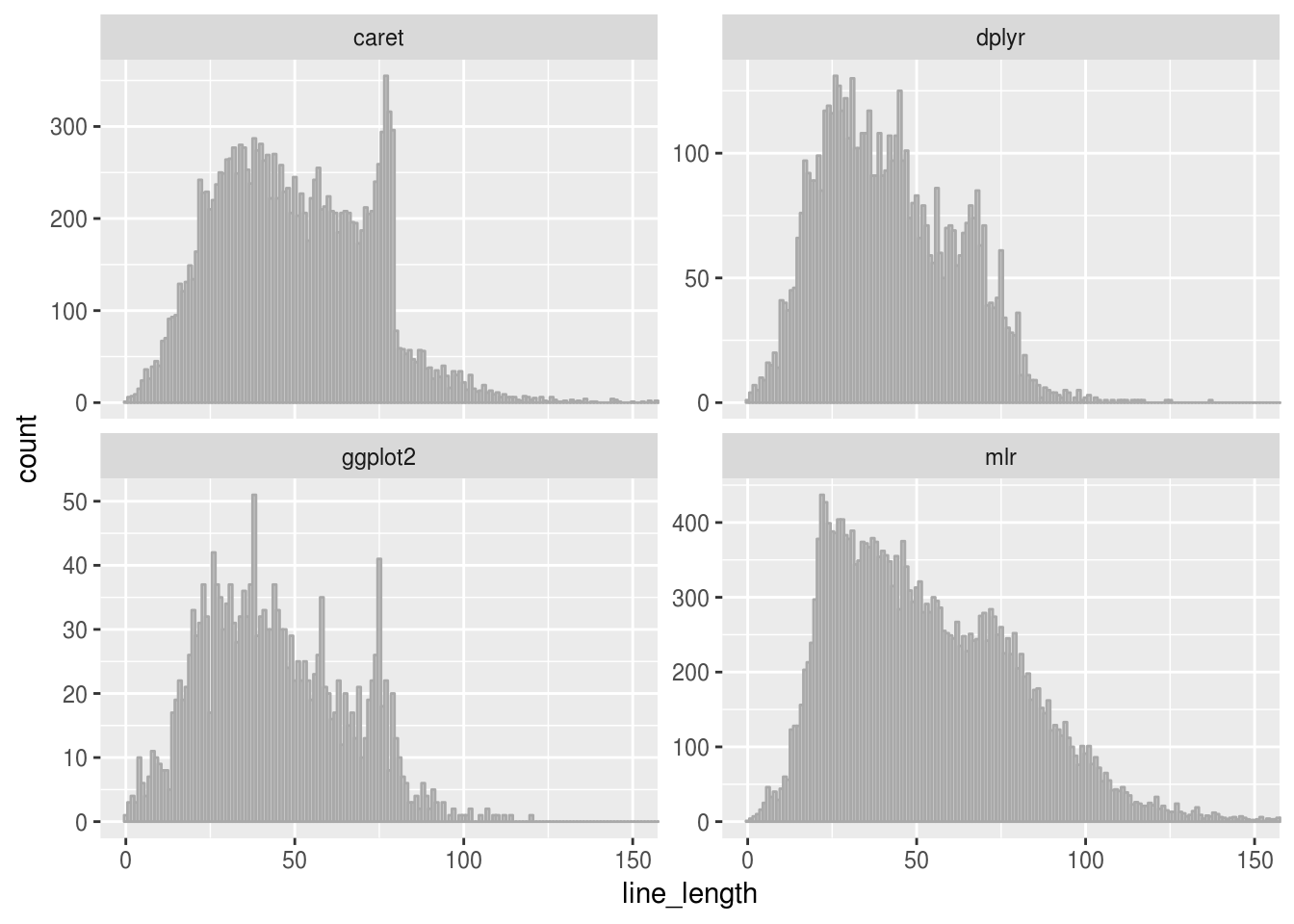
From this visualization, we can observe the following:
The tidyverse packages ggplot2 and dplyr apparently don’t enforce a limit of the line length; the histograms of line length are quite similar.
The machine learning framework mlr does not enforce a limit on line length. There is a little bump in the distribution around a line length of 75, but mlr apparently allows (and uses) much longer lines.
The second machine learning framework, caret, is notably different from mlr: Here, we observe a very similar pattern to packages from the python world, where a strict line lenght is enforced. Longer lines occur, but there is a very sharp decline at approximately 80 caracters. Apparently, lines in caret are supposed to be shorter than 79 (or 80) characters. This might either be the result of a style guide (which I did not find with a quick search), or the developer uses an editor setting which enforces this line length limit.
Discussion and conclusion
We have analyzed the distribution of line lenghts in the source code of several R packages.
In two packages from the tidyverse, we have observed similarites in the line length distribution. These packages have both been written by the same developer, suggesting that the (main) developer has a distinct coding habit. We have further analyzed two machine learning frameworks and have found striking differences: The machine learning framework caret appears to enforce a character limit on the line length, wheras the machine learning framework mlr allows more liberties for its developers.
In further work, one could attempt to quantify similarities and differences of line length distributions. This would allow to cluster packages and possibly to attribute packages to developers (or groups of developers). Other measures for similarity may be found by text analysis with tidy text tools (although I am not sure whether these tools can be used in a meaningful way for source code). Of course, it is straightforward to extend the present analysis to additional packages.
Personally, I am not sure about the benefits of a strict line length limit. While line lengths of approximately 45-90 characters are a typographical standard, I am not sure whether enforcing such line lengths leads to better readibility of code. While shorter lines are generally easier to read, it may occassionaly be better to write a long line than enforcing an artifical line break.
On a personal note: I enjoyed this analysis very much, it was an excellent exeRcise, and I believe it has considerably improved my R programming skills. In particular, I would like to thank Jake VanderPlas for inspiration and his exceptional blog.
I’m looking forward to your comments!